The Open API of Systembolaget

Data

The data consists of three XML trees; one for product data, one for store data, and one for stock data. The product data contains products attributes such as product type, price, country of origin, and alcoholic content. The store data contains store attributes such as location and opening hours. The stock data consists of only two columns indicating in which stores specific products currently are in stock. I will now show you how to fetch all three XML trees and eventually join them into one dataset using R.

Product and Store Data

We begin by fetching the product and store data. As seen below, the xml2 package is used read the XML trees into R and the XML package to parse them into dataframes.

library(xml2)
library(XML)
 
#Read store data
store_xml <- read_xml("https://www.systembolaget.se/api/assortment/stores/xml")
stores <- xmlToDataFrame(nodes = getNodeSet(xmlParse(store_xml), "//ButikOmbud"))
  
#Read product data
product_xml <- read_xml("https://www.systembolaget.se/api/assortment/products/xml")
products <- xmlToDataFrame(nodes = getNodeSet(xmlParse(product_xml), "//artikel"))

Since the column names are in Swedish and since not all columns will be needed for data analysis, let’s rename usable columns into English. The values will, however, remain in Swedish. By default, all values will be formatted as characters. Therefore, some of the columns in the product data, e.g., price columns, need to be converted into numeric. Fortunately, this can easily be done using sapply().

library(tidyverse)

#Select store data for analysis#
stores <- stores %>% select(
  STORE_TYPE=Typ, 
  STORE_CODE=Nr, 
  STORE_NAME=Namn, 
  STORE_STREET=Address1,
  STORE_ZIP=Address3, 
  STORE_CITY=Address4, 
  STORE_REGION=Address5
  )

#Select product data for analysis
 products <- products %>% select(
  PRODUCT_ID=nr, 
  PRODUCT_VNR=Varnummer, 
  PRODUCT_NAME=Namn, 
  PRODUCT_NAME_2=Namn2,
  PRODUCT_PRICE_VAT=Prisinklmoms, 
  PRODUCT_ML=Volymiml, 
  PRODUCT_PRICE_L=PrisPerLiter,
  PRODUCT_SALES_START=Saljstart, 
  PRODUCT_TYPE=Varugrupp, 
  PRODUCT_TYPE_2=Typ,
  PRODUCT_STYLE=Stil, 
  PRODUCT_PACKAGE=Forpackning, 
  PRODUCT_SEAL=Forslutning,
  PRODUCT_ORIGIN=Ursprung, 
  PRODUCT_ORIGIN_COUNTRY=Ursprunglandnamn, 
  PRODUCT_PRODUCER=Producent, 
  PRODUCT_SUPPLIER=Leverantor, 
  PRODUCT_YEAR=Argang,
  PRODUCT_ALCOHOL=Alkoholhalt, 
  PRODUCT_SORTIMENT=Sortiment, 
  PRODUCT_SORTIMENT_TEXT=SortimentText, 
  PRODUCT_ORGANIC=Ekologisk
  )
 
#Convert some columns to numeric
products[, c(5,6,7,18,22)] <- sapply(products[, c(5,6,7,18,22)], as.numeric)

Stock Data

Fetching the stock data is a bit trickier. Again, I use xml2 to read the XML tree into R. In the second stop, I create a list of the children nodes and extract only numeric values from this list. The reason for this is that store codes and product ID’s are both numeric. The first number in the list (called values below) is the store code, the remaining numbers are product ID’s. Note that the length varies across rows, i.e., stores. I use the tidyr package to transform the list into a long tibble.

library(stringr)

#Read XML from Systembolaget
store_assortment_xml <- read_xml("https://www.systembolaget.se/api/assortment/stock/xml")
  
#Transform the XML into a tibble
assortment_tibble <- store_assortment_xml %>% xml_children() %>% tibble()
  
#Extract all numeric values from the XML (first is store code; rest article ID's)
values <- str_extract_all(assortment_tibble$.,"\\(?[0-9,.]+\\)?") 
  
#Function to transform this to a long tibble
get_assortment_by_store <- function(store) {
  assortment_length <- length(values[[store]])
  tmp_tibble <- tibble(
    PRODUCT_ID=values[[store]][2:assortment_length],
    STORE_CODE=values[[store]][1]
  )
}
  
#Run function
store_assortment <- map_df(2:length(values), get_assortment_by_store)

The stock data is useless without product and store attributes. As a final step, all three tibbles are joined together. Note that I use the inner_join() function to only consider stores and products for which there is complete data. The dataset is now ready for analysis.

#Add store/product data to store assortment data
store_assortment <- store_assortment %>% 
  inner_join(stores, by="STORE_CODE") %>% 
  inner_join(products, by="PRODUCT_ID")
 
#Get a glimpse of the final dataset
glimpse(store_assortment)

## Observations: 578,244
## Variables: 29
## $ PRODUCT_ID             <chr> "1192003", "7660201", "9975101", "14111...
## $ STORE_CODE             <chr> "0102", "0102", "0102", "0102", "0102",...
## $ STORE_TYPE             <chr> "Butik", "Butik", "Butik", "Butik", "Bu...
## $ STORE_NAME             <chr> "Fältöversten", "Fältöversten", "Fältöv...
## $ STORE_STREET           <chr> "Karlaplan 13", "Karlaplan 13", "Karlap...
## $ STORE_ZIP              <chr> "115 20", "115 20", "115 20", "115 20",...
## $ STORE_CITY             <chr> "STOCKHOLM", "STOCKHOLM", "STOCKHOLM", ...
## $ STORE_REGION           <chr> "Stockholms län", "Stockholms län", "St...
## $ PRODUCT_VNR            <chr> "11920", "76602", "99751", "1411", "894...
## $ PRODUCT_NAME           <chr> "1664 Blanc Non-Alco", "Côtes du Rhône"...
## $ PRODUCT_NAME_2         <chr> "", "Reserve Blanc", "Wild Ferment", "S...
## $ PRODUCT_PRICE_VAT      <dbl> 10.9, 79.0, 189.0, 7.9, 179.0, 16.9, 23...
## $ PRODUCT_ML             <dbl> 250, 750, 750, 330, 700, 330, 500, 750,...
## $ PRODUCT_PRICE_L        <dbl> 43.60, 105.33, 252.00, 23.94, 255.71, 5...
## $ PRODUCT_SALES_START    <chr> "2017-06-01", "2017-03-27", "2017-09-08...
## $ PRODUCT_TYPE           <chr> "Alkoholfritt", "Vitt vin", "Vitt vin",...
## $ PRODUCT_TYPE_2         <chr> "Öl", "Druvigt & Blommigt", "Fylligt & ...
## $ PRODUCT_STYLE          <chr> "", "", "", "Internationell stil", "", ...
## $ PRODUCT_PACKAGE        <chr> "Flaska", "Flaska", "Flaska", "Burk", "...
## $ PRODUCT_SEAL           <chr> "", "Skruvkapsyl", "Plast", "", "", "",...
## $ PRODUCT_ORIGIN         <chr> "", "Rhonedalen", "Santorini", "Kalmar ...
## $ PRODUCT_ORIGIN_COUNTRY <chr> "Frankrike", "Frankrike", "Grekland", "...
## $ PRODUCT_PRODUCER       <chr> "Kronenbourg", "Pellerin", "Gaia", "Åbr...
## $ PRODUCT_SUPPLIER       <chr> "Carlsberg Sverige AB", "Giertz Vinimpo...
## $ PRODUCT_YEAR           <dbl> NA, 2016, 2016, NA, NA, NA, NA, NA, 201...
## $ PRODUCT_ALCOHOL        <chr> "0.50%", "13.00%", "13.00%", "5.20%", "...
## $ PRODUCT_SORTIMENT      <chr> "FSÖ", "FS", "TSE", "FS", "FS", "FS", "...
## $ PRODUCT_SORTIMENT_TEXT <chr> "Ordinarie sortiment", "Ordinarie sorti...
## $ PRODUCT_ORGANIC        <dbl> 0, 0, 0, 0, 0, 0, 0, 0, 0, 0, 0, 0, 0, ...

k-Means Clustering of Stores

The stores of Systembolaget are quite sterile, in my opinion. They all look the same, the opening hours are more of less the same, and the staff have been trained in exactly the same, politically correct way. One thing that differs across stores, though, is the assortment. This made me wonder. How many types of Systembolaget stores are there? In this section, I will investigate the question through k-means clustering.

Finding the Optimal k

For simplicity, I will focus on (i) assortment width as measured by number of distinct products in the store and (ii) the general price level as measured by the average liter price in the store. First we need to decide on an optimal k, i.e., an optimal number of clusters. We’ll use the elbow approach for this. As illustrated below, I consider k \(\in\) {1, 2, …, 15}.

#Calculate assortment width (no. of articles) and average price per store
assortment_size <- store_assortment %>% 
  group_by(STORE_CODE) %>% 
  summarise(ARTICLES=sum(n()), PRICE=mean(PRODUCT_PRICE_L)) %>% 
  ungroup() %>% 
  select(-STORE_CODE)

#Function to calculate the average within cluster distance to centroid
elbow_k <- function(k) {
  store_clusters <- kmeans(assortment_size, k)
  tmp <- tibble(withinss=sum(store_clusters$withinss), K=k)
}

#Get the data from the function
elbow_data <- map_df(1:15, elbow_k)

#Plot the data
ggplot(elbow_data, aes(x=K, y=withinss)) + 
  geom_point(color="#0b7b3e", size=4) +
  geom_point(shape=1, size=4) +
  geom_line() + 
  theme_minimal()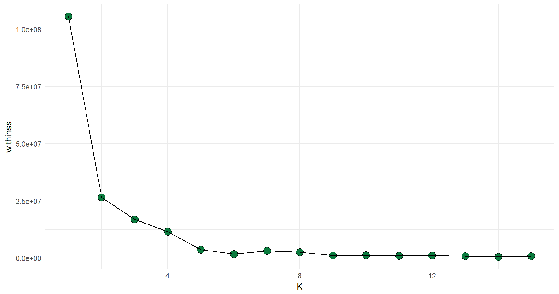

This graph illustrates the average within cluster distance to centroid for different levels of k. A low number indicates a homogenous cluster as most data points (in this case: stores) are fairly close to the average values of all variables within the cluster.

Plotting the Stores

To continue the analysis, we chose k=4 as more clusters will not decrease the undesirable heterogeneity that much. After that, each store is assigned to one of the four clusters, as given be the code below. Before plotting it all, let’s begin by examining the four centroids.

#Let's pick four clusters
k4 <- kmeans(assortment_size, 4)

#Assign a cluster to each store
assortment_size$CLUSTER <- k4$cluster

#Identifying the four centroids
k4$centers

##   ARTICLES    PRICE
## 1 1032.712 174.5363
## 2 1543.486 190.5071
## 3  593.680 163.1905
## 4 2047.671 203.1835

Finally, I plot all stores with respect to its assortment width, its average price, and its cluster:

#Plot all stores w.r.t. no. of. articles, avg. price and its cluster
ggplot(assortment_size, aes(x=ARTICLES, y=PRICE, color=as.character(CLUSTER))) + 
  geom_point() +
  labs(x="Assortment Width (# of Aritcles)", y="Average Price (SEK)", color="Cluster") +
  theme_minimal() +
  scale_color_manual(values=c("#0b7b3e", "#fed401", "grey", "black"))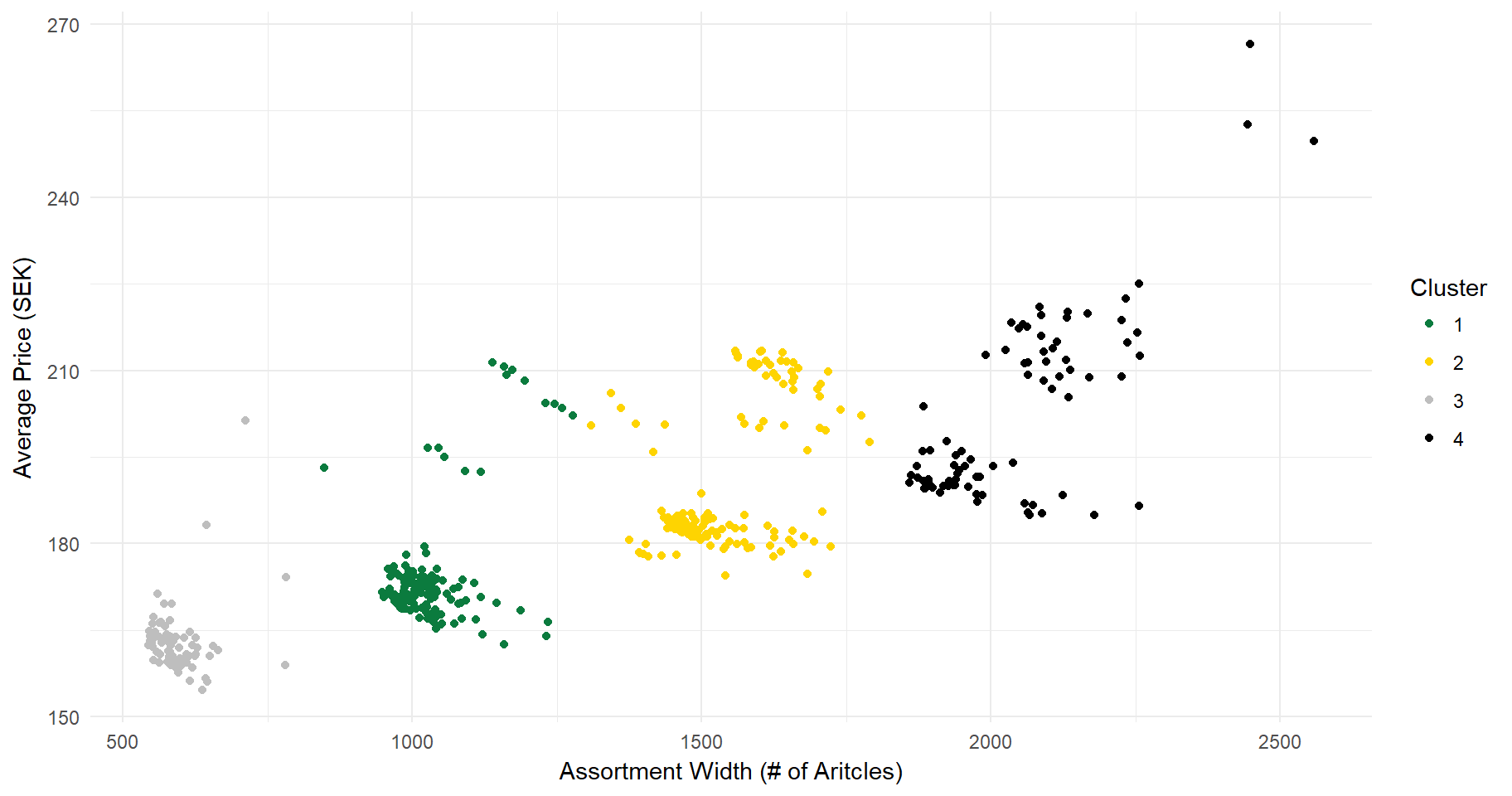

Conclusions

While this approach is rather simplistic, it certainly does look like Systembolaget carefully plans their stores so that they fit into any of the four categories. Stores typically have an assortment of 600, 1,100, 1,600, or 2,100 distinct articles. Interestingly, the assortmertment width across the four store categories increases in increments of 500 distinct articles. The average product prices is higher in stores with a larger assortment. Most likely, larger stores have the base sortiment (i.e., products typically found in the smaller stores), and some additional premium products.